Tutorial 1g: Recording membrane potentials
In the previous part of this tutorial, we plotted a raster plot of the firing times of the network. In this tutorial, we introduce a way to record the value of the membrane potential for a neuron during the simulation, and plot it. We continue as before:
from brian import *

tau = 20 * msecond        # membrane time constant
Vt = -50 * mvolt          # spike threshold
Vr = -60 * mvolt          # reset value
El = -49 * mvolt          # resting potential (same as the reset)
psp = 0.5 * mvolt         # postsynaptic potential size

G = NeuronGroup(N=40, model='dV/dt = -(V-El)/tau : volt',
              threshold=Vt, reset=Vr)

C = Connection(G, G)
C.connect_random(sparseness=0.1, weight=psp)
This time we won’t record the spikes.
Recording states
Now we introduce a second type of monitor, the StateMonitor.
The first argument is the group to monitor, and the second is
the state variable to monitor. The keyword record can be
an integer, list or the value True. If it is an integer i,
the monitor will record the state of the variable for neuron i.
If it’s a list of integers, it will record the states for
each neuron in the list. If it’s set to True it will record
for all the neurons in the group.
M = StateMonitor(G, 'V', record=0)
And then we continue as before:
G.V = Vr + rand(40) * (Vt - Vr)
But this time we run it for a shorter time so we can look at the output in more detail:
run(200 * msecond)
Having run the simulation, we plot the results using the
plot command from PyLab which has the same syntax as the Matlab
plot` command, i.e. plot(xvals,yvals,...). The StateMonitor
monitors the times at which it monitored a value in the
array M.times, and the values in the array M[0]. The notation
M[i] means the array of values of the monitored state
variable for neuron i.
In the following lines, we scale the times so that they’re
measured in ms and the values so that they’re measured in
mV. We also label the plot using PyLab’s xlabel, ylabel and
title functions, which again mimic the Matlab equivalents.
plot(M.times / ms, M[0] / mV)
xlabel('Time (in ms)')
ylabel('Membrane potential (in mV)')
title('Membrane potential for neuron 0')
show()
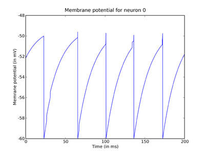
You can clearly see the leaky integration exponential decay toward the resting potential, as well as the jumps when a spike was received.