Tutorial 1f: Recording spikes
In the previous part of the tutorial, we defined a network with not entirely trivial behaviour, and printed the number of spikes. In this part, we’ll record every spike that the network generates and display a raster plot of them. We start as before:
from brian import *

tau = 20 * msecond        # membrane time constant
Vt = -50 * mvolt          # spike threshold
Vr = -60 * mvolt          # reset value
El = -49 * mvolt          # resting potential (same as the reset)
psp = 0.5 * mvolt         # postsynaptic potential size

G = NeuronGroup(N=40, model='dV/dt = -(V-El)/tau : volt',
              threshold=Vt, reset=Vr)

C = Connection(G, G)
C.connect_random(sparseness=0.1, weight=psp)

M = SpikeMonitor(G)

G.V = Vr + rand(40) * (Vt - Vr)

run(1 * second)

print M.nspikes
Having run the network, we simply use the raster_plot() function
provided by Brian. After creating plots, we have to use the
show() function to display them. This function is from the
PyLab module that Brian uses for its built in plotting
routines.
raster_plot()
show()
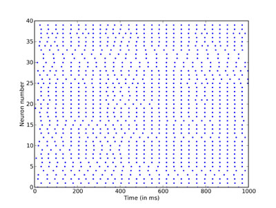
As you can see, despite having introduced some randomness into our network, the output is very regular indeed. In the next part we introduce one more way to plot the output of a network.