Brian hears
See also
User guide for Brian hears.
- brian.hears.set_default_samplerate(samplerate)
Sets the default samplerate for Brian hears objects, by default 44.1 kHz.
Sounds
- class brian.hears.Sound
Class for working with sounds, including loading/saving, manipulating and playing.
For an overview, see Sounds.
Initialisation
The following arguments are used to initialise a sound object
- data
- Can be a filename, an array, a function or a sequence (list or tuple). If its a filename, the sound file (WAV or AIFF) will be loaded. If its an array, it should have shape (nsamples, nchannels). If its a function, it should be a function f(t). If its a sequence, the items in the sequence can be filenames, functions, arrays or Sound objects. The output will be a multi-channel sound with channels the corresponding sound for each element of the sequence.
- samplerate=None
- The samplerate, if necessary, will use the default (for an array or function) or the samplerate of the data (for a filename).
- duration=None
- The duration of the sound, if initialising with a function.
Loading, saving and playing
- static load(filename)
Load the file given by filename and returns a Sound object. Sound file can be either a .wav or a .aif file.
- save(filename, normalise=False, samplewidth=2)
Save the sound as a WAV.
If the normalise keyword is set to True, the amplitude of the sound will be normalised to 1. The samplewidth keyword can be 1 or 2 to save the data as 8 or 16 bit samples.
- play(normalise=False, sleep=False)
Plays the sound (normalised to avoid clipping if required). If sleep=True then the function will wait until the sound has finished playing before returning.
Properties
- duration
The length of the sound in seconds.
- nsamples
The number of samples in the sound.
- nchannels
The number of channels in the sound.
- times
An array of times (in seconds) corresponding to each sample.
- left
The left channel for a stereo sound.
- right
The right channel for a stereo sound.
- channel(n)
Returns the nth channel of the sound.
Generating sounds
All sound generating methods can be used with durations arguments in samples (int) or units (e.g. 500*ms). One can also set the number of channels by setting the keyword argument nchannels to the desired value. Notice that for noise the channels will be generated independantly.
- static tone(*args, **kwds)
Returns a pure tone at frequency for duration, using the default samplerate or the given one. The frequency and phase parameters can be single values, in which case multiple channels can be specified with the nchannels argument, or they can be sequences (lists/tuples/arrays) in which case there is one frequency or phase for each channel.
- static whitenoise(*args, **kwds)
Returns a white noise. If the samplerate is not specified, the global default value will be used.
- static powerlawnoise(*args, **kwds)
Returns a power-law noise for the given duration. Spectral density per unit of bandwidth scales as 1/(f**alpha).
Sample usage:
noise = powerlawnoise(200*ms, 1, samplerate=44100*Hz)
Arguments:
- duration
- Duration of the desired output.
- alpha
- Power law exponent.
- samplerate
- Desired output samplerate
- static brownnoise(*args, **kwds)
Returns brown noise, i.e powerlawnoise() with alpha=2
- static pinknoise(*args, **kwds)
Returns pink noise, i.e powerlawnoise() with alpha=1
- static silence(*args, **kwds)
Returns a silent, zero sound for the given duration. Set nchannels to set the number of channels.
- static click(*args, **kwds)
Returns a click of the given duration.
If peak is not specified, the amplitude will be 1, otherwise peak refers to the peak dB SPL of the click, according to the formula 28e-6*10**(peak/20.).
- static harmoniccomplex(*args, **kwds)
Returns a harmonic complex composed of pure tones at integer multiples of the fundamental frequency f0. The amplitude and phase keywords can be set to either a single value or an array of values. In the former case the value is set for all harmonics, and harmonics up to the sampling frequency are generated. In the latter each harmonic parameter is set separately, and the number of harmonics generated corresponds to the length of the array.
- static vowel(*args, **kwds)
Returns an artifically created spoken vowel sound (following the source-filter model of speech production) with a given pitch.
The vowel can be specified by either providing vowel as a string (‘a’, ‘i’ or ‘u’) or by setting formants to a sequence of formant frequencies.
The returned sound is normalized to a maximum amplitude of 1.
The implementation is based on the MakeVowel function written by Richard O. Duda, part of the Auditory Toolbox for Matlab by Malcolm Slaney: http://cobweb.ecn.purdue.edu/~malcolm/interval/1998-010/
Timing and sequencing
- static sequence(*sounds, samplerate=None)
Returns the sequence of sounds in the list sounds joined together
- repeat(n)
Repeats the sound n times
- extended(duration)
Returns the Sound with length extended by the given duration, which can be the number of samples or a length of time in seconds.
- shifted(duration, fractional=False, filter_length=2048)
Returns the sound delayed by duration, which can be the number of samples or a length of time in seconds. Normally, only integer numbers of samples will be used, but if fractional=True then the filtering method from http://www.labbookpages.co.uk/audio/beamforming/fractionalDelay.html will be used (introducing some small numerical errors). With this method, you can specify the filter_length, larger values are slower but more accurate, especially at higher frequencies. The large default value of 2048 samples provides good accuracy for sounds with frequencies above 20 Hz, but not for lower frequency sounds. If you are restricted to high frequency sounds, a smaller value will be more efficient. Note that if fractional=True then duration is assumed to be a time not a number of samples.
- resized(L)
Returns the Sound with length extended (or contracted) to have L samples.
Slicing
One can slice sound objects in various ways, for example sound[100*ms:200*ms] returns the part of the sound between 100 ms and 200 ms (not including the right hand end point). If the sound is less than 200 ms long it will be zero padded. You can also set values using slicing, e.g. sound[:50*ms] = 0 will silence the first 50 ms of the sound. The syntax is the same as usual for Python slicing. In addition, you can select a subset of the channels by doing, for example, sound[:, -5:] would be the last 5 channels. For time indices, either times or samples can be given, e.g. sound[:100] gives the first 100 samples. In addition, steps can be used for example to reverse a sound as sound[::-1].
Arithmetic operations
Standard arithemetical operations and numpy functions work as you would expect with sounds, e.g. sound1+sound2, 3*sound or abs(sound).
Level
- level
Can be used to get or set the level of a sound, which should be in dB. For single channel sounds a value in dB is used, for multiple channel sounds a value in dB can be used for setting the level (all channels will be set to the same level), or a list/tuple/array of levels. It is assumed that the unit of the sound is Pascals.
- atlevel(level)
Returns the sound at the given level in dB SPL (RMS) assuming array is in Pascals. level should be a value in dB, or a tuple of levels, one for each channel.
- maxlevel
Can be used to set or get the maximum level of a sound. For mono sounds, this is the same as the level, but for multichannel sounds it is the maximum level across the channels. Relative level differences will be preserved. The specified level should be a value in dB, and it is assumed that the unit of the sound is Pascals.
- atmaxlevel(level)
Returns the sound with the maximum level across channels set to the given level. Relative level differences will be preserved. The specified level should be a value in dB and it is assumed that the unit of the sound is Pascals.
Ramping
- ramp(when='onset', duration=10.0 * msecond, envelope=None, inplace=True)
Adds a ramp on/off to the sound
- when='onset'
- Can take values ‘onset’, ‘offset’ or ‘both’
- duration=10*ms
- The time over which the ramping happens
- envelope
- A ramping function, if not specified uses sin(pi*t/2)**2. The function should be a function of one variable t ranging from 0 to 1, and should increase from f(0)=0 to f(0)=1. The reverse is applied for the offset ramp.
- inplace
- Whether to apply ramping to current sound or return a new array.
- ramped(*args, **kwds)
Returns a ramped version of the sound (see Sound.ramp()).
Plotting
- spectrogram(low=None, high=None, log_power=True, other=None, **kwds)
Plots a spectrogram of the sound
Arguments:
- low=None, high=None
- If these are left unspecified, it shows the full spectrogram, otherwise it shows only between low and high in Hz.
- log_power=True
- If True the colour represents the log of the power.
- **kwds
- Are passed to Pylab’s specgram command.
Returns the values returned by pylab’s specgram, namely (pxx, freqs, bins, im) where pxx is a 2D array of powers, freqs is the corresponding frequencies, bins are the time bins, and im is the image axis.
- spectrum(*args, **kwds)
Returns the spectrum of the sound and optionally plots it.
Arguments:
- low, high
- If these are left unspecified, it shows the full spectrum, otherwise it shows only between low and high in Hz.
- log_power=True
- If True it returns the log of the power.
- display=False
- Whether to plot the output.
Returns (Z, freqs, phase) where Z is a 1D array of powers, freqs is the corresponding frequencies, phase is the unwrapped phase of spectrum.
- brian.hears.savesound(sound, filename, normalise=False, samplewidth=2)
Save the sound as a WAV.
If the normalise keyword is set to True, the amplitude of the sound will be normalised to 1. The samplewidth keyword can be 1 or 2 to save the data as 8 or 16 bit samples.
- brian.hears.loadsound(filename)
Load the file given by filename and returns a Sound object. Sound file can be either a .wav or a .aif file.
- brian.hears.play(*sounds, normalise=False, sleep=False)
Plays the sound (normalised to avoid clipping if required). If sleep=True then the function will wait until the sound has finished playing before returning.
- brian.hears.whitenoise(*args, **kwds)
Returns a white noise. If the samplerate is not specified, the global default value will be used.
- brian.hears.powerlawnoise(*args, **kwds)
Returns a power-law noise for the given duration. Spectral density per unit of bandwidth scales as 1/(f**alpha).
Sample usage:
noise = powerlawnoise(200*ms, 1, samplerate=44100*Hz)
Arguments:
- duration
- Duration of the desired output.
- alpha
- Power law exponent.
- samplerate
- Desired output samplerate
- brian.hears.brownnoise(*args, **kwds)
Returns brown noise, i.e powerlawnoise() with alpha=2
- brian.hears.pinknoise(*args, **kwds)
Returns pink noise, i.e powerlawnoise() with alpha=1
- brian.hears.irns(*args, **kwds)
Returns an IRN_S noise. The iterated ripple noise is obtained trough a cascade of gain and delay filtering. For more details: see Yost 1996 or chapter 15 in Hartman Sound Signal Sensation.
- brian.hears.irno(*args, **kwds)
Returns an IRN_O noise. The iterated ripple noise is obtained many attenuated and delayed version of the original broadband noise. For more details: see Yost 1996 or chapter 15 in Hartman Sound Signal Sensation.
- brian.hears.tone(*args, **kwds)
Returns a pure tone at frequency for duration, using the default samplerate or the given one. The frequency and phase parameters can be single values, in which case multiple channels can be specified with the nchannels argument, or they can be sequences (lists/tuples/arrays) in which case there is one frequency or phase for each channel.
- brian.hears.click(*args, **kwds)
Returns a click of the given duration.
If peak is not specified, the amplitude will be 1, otherwise peak refers to the peak dB SPL of the click, according to the formula 28e-6*10**(peak/20.).
- brian.hears.clicks(*args, **kwds)
Returns a series of n clicks (see click()) separated by interval.
- brian.hears.harmoniccomplex(*args, **kwds)
Returns a harmonic complex composed of pure tones at integer multiples of the fundamental frequency f0. The amplitude and phase keywords can be set to either a single value or an array of values. In the former case the value is set for all harmonics, and harmonics up to the sampling frequency are generated. In the latter each harmonic parameter is set separately, and the number of harmonics generated corresponds to the length of the array.
- brian.hears.silence(*args, **kwds)
Returns a silent, zero sound for the given duration. Set nchannels to set the number of channels.
- brian.hears.sequence(*sounds, samplerate=None)
Returns the sequence of sounds in the list sounds joined together
Filterbanks
- class brian.hears.LinearFilterbank(source, b, a)
Generalised linear filterbank
Initialisation arguments:
- source
- The input to the filterbank, must have the same number of channels or just a single channel. In the latter case, the channels will be replicated.
- b, a
- The coeffs b, a must be of shape (nchannels, m) or (nchannels, m, p). Here m is the order of the filters, and p is the number of filters in a chain (first you apply [:, :, 0], then [:, :, 1], etc.).
The filter parameters are stored in the modifiable attributes filt_b, filt_a and filt_state (the variable z in the section below).
Has one method:
- decascade(ncascade=1)
Reduces cascades of low order filters into smaller cascades of high order filters.
ncascade is the number of cascaded filters to use, which should be a divisor of the original number.
Note that higher order filters are often numerically unstable.
Notes
These notes adapted from scipy’s lfilter() function.
The filterbank is implemented as a direct II transposed structure. This means that for a single channel and element of the filter cascade, the output y for an input x is defined by:
a[0]*y[m] = b[0]*x[m] + b[1]*x[m-1] + ... + b[m]*x[0]
                      - a[1]*y[m-1] - ... - a[m]*y[0]
using the following difference equations:
y[i] = b[0]*x[i] + z[0,i-1]
z[0,i] = b[1]*x[i] + z[1,i-1] - a[1]*y[i]
...
z[m-3,i] = b[m-2]*x[i] + z[m-2,i-1] - a[m-2]*y[i]
z[m-2,i] = b[m-1]*x[i] - a[m-1]*y[i]
where i is the output sample number.
The rational transfer function describing this filter in the z-transform domain is:
                    -1              -nb
        b[0] + b[1]z  + ... + b[m] z
Y(z) = --------------------------------- X(z)
                    -1              -na
        a[0] + a[1]z  + ... + a[m] z
- class brian.hears.FIRFilterbank(source, impulse_response, use_linearfilterbank=False, minimum_buffer_size=None)
Finite impulse response filterbank
Initialisation parameters:
- source
- Source sound or filterbank.
- impulse_response
- Either a 1D array providing a single impulse response applied to every input channel, or a 2D array of shape (nchannels, ir_length) for ir_length the number of samples in the impulse response. Note that if you are using a multichannel sound x as a set of impulse responses, the array should be impulse_response=array(x.T).
- minimum_buffer_size=None
- If specified, gives a minimum size to the buffer. By default, for the FFT convolution based implementation of FIRFilterbank, the minimum buffer size will be 3*ir_length. For maximum efficiency with FFTs, buffer_size+ir_length should be a power of 2 (otherwise there will be some zero padding), and buffer_size should be as large as possible.
- class brian.hears.RestructureFilterbank(source, numrepeat=1, type='serial', numtile=1, indexmapping=None)
Filterbank used to restructure channels, including repeating and interleaving.
Standard forms of usage:
Repeat mono source N times:
RestructureFilterbank(source, N)
For a stereo source, N copies of the left channel followed by N copies of the right channel:
RestructureFilterbank(source, N)
For a stereo source, N copies of the channels tiled as LRLRLR...LR:
RestructureFilterbank(source, numtile=N)
For two stereo sources AB and CD, join them together in serial to form the output channels in order ABCD:
RestructureFilterbank((AB, CD))
For two stereo sources AB and CD, join them together interleaved to form the output channels in order ACBD:
RestructureFilterbank((AB, CD), type='interleave')
These arguments can also be combined together, for example to AB and CD into output channels AABBCCDDAABBCCDDAABBCCDD:
RestructureFilterbank((AB, CD), 2, 'serial', 3)
The three arguments are the number of repeats before joining, the joining type (‘serial’ or ‘interleave’) and the number of tilings after joining. See below for details.
Initialise arguments:
- source
- Input source or list of sources.
- numrepeat=1
- Number of times each channel in each of the input sources is repeated before mixing the source channels. For example, with repeat=2 an input source with channels AB will be repeated to form AABB
- type='serial'
- The method for joining the source channels, the options are 'serial' to join the channels in series, or 'interleave' to interleave them. In the case of 'interleave', each source must have the same number of channels. An example of serial, if the input sources are abc and def the output would be abcdef. For interleave, the output would be adbecf.
- numtile=1
- The number of times the joined channels are tiled, so if the joined channels are ABC and numtile=3 the output will be ABCABCABC.
- indexmapping=None
- Instead of specifying the restructuring via numrepeat, type, numtile you can directly give the mapping of input indices to output indices. So for a single stereo source input, indexmapping=[1,0] would reverse left and right. Similarly, with two mono sources, indexmapping=[1,0] would have channel 0 of the output correspond to source 1 and channel 1 of the output corresponding to source 0. This is because the indices are counted in order of channels starting from the first source and continuing to the last. For example, suppose you had two sources, each consisting of a stereo sound, say source 0 was AB and source 1 was CD then indexmapping=[1, 0, 3, 2] would swap the left and right of each source, but leave the order of the sources the same, i.e. the output would be BADC.
- class brian.hears.Join(*sources)
Filterbank that joins the channels of its inputs in series, e.g. with two input sources with channels AB and CD respectively, the output would have channels ABCD. You can initialise with multiple sources separated by commas, or by passing a list of sources.
- class brian.hears.Interleave(*sources)
Filterbank that interleaves the channels of its inputs, e.g. with two input sources with channels AB and CD respectively, the output would have channels ACBD. You can initialise with multiple sources separated by commas, or by passing a list of sources.
- class brian.hears.Repeat(source, numrepeat)
Filterbank that repeats each channel from its input, e.g. with 3 repeats channels ABC would map to AAABBBCCC.
- class brian.hears.Tile(source, numtile)
Filterbank that tiles the channels from its input, e.g. with 3 tiles channels ABC would map to ABCABCABC.
- class brian.hears.FunctionFilterbank(source, func, nchannels=None, **params)
Filterbank that just applies a given function. The function should take as many arguments as there are sources.
For example, to half-wave rectify inputs:
FunctionFilterbank(source, lambda x: clip(x, 0, Inf))
The syntax lambda x: clip(x, 0, Inf) defines a function object that takes a single argument x and returns clip(x, 0, Inf). The numpy function clip(x, low, high) returns the values of x clipped between low and high (so if x<low it returns low, if x>high it returns high, otherwise it returns x). The symbol Inf means infinity, i.e. no clipping of positive values.
Technical details
Note that functions should operate on arrays, in particular on 2D buffered segments, which are arrays of shape (bufsize, nchannels). Typically, most standard functions from numpy will work element-wise.
If you want a filterbank that changes the shape of the input (e.g. changes the number of channels), set the nchannels keyword argument to the number of output channels.
- class brian.hears.SumFilterbank(source, weights=None)
Sum filterbanks together with given weight vectors.
For example, to take the sum of two filterbanks:
SumFilterbank((fb1, fb2))
To take the difference:
SumFilterbank((fb1, fb2), (1, -1))
- class brian.hears.DoNothingFilterbank(source)
Filterbank that does nothing to its input.
Useful for removing a set of filters without having to rewrite your code. Can also be used for simply writing compound derived classes. For example, if you want a compound Filterbank that does AFilterbank and then BFilterbank, but you want to encapsulate that into a single class, you could do:
class ABFilterbank(DoNothingFilterbank):
    def __init__(self, source):
        a = AFilterbank(source)
        b = BFilterbank(a)
        DoNothingFilterbank.__init__(self, b)
However, a more general way of writing compound filterbanks is to use CombinedFilterbank.
- class brian.hears.ControlFilterbank(source, inputs, targets, updater, max_interval=None)
Filterbank that can be used for controlling behaviour at runtime
Typically, this class is used to implement a control path in an auditory model, modifying some filterbank parameters based on the output of other filterbanks (or the same ones).
The controller has a set of input filterbanks whose output values are used to modify a set of output filterbanks. The update is done by a user specified function or class which is passed these output values. The controller should be inserted as the last bank in a chain.
Initialisation arguments:
- source
- The source filterbank, the values from this are used unmodified as the output of this filterbank.
- inputs
- Either a single filterbank, or sequence of filterbanks which are used as inputs to the updater.
- targets
- The filterbank or sequence of filterbanks that are modified by the updater.
- updater
- The function or class which does the updating, see below.
- max_interval
- If specified, ensures that the updater is called at least as often as this interval (but it may be called more often). Can be specified as a time or a number of samples.
The updater
The updater argument can be either a function or class instance. If it is a function, it should have a form like:
# A single input
def updater(input):
    ...

# Two inputs
def updater(input1, input2):
    ...

# Arbitrary number of inputs
def updater(*inputs):
    ...
Each argument input to the function is a numpy array of shape (numsamples, numchannels) where numsamples is the number of samples just computed, and numchannels is the number of channels in the corresponding filterbank. The function is not restricted in what it can do with these inputs.
Functions can be used to implement relatively simple controllers, but for more complicated situations you may want to maintain some state variables for example, and in this case you can use a class. The object updater should be an instance of a class that defines the __call__ method (with the same syntax as above for functions). In addition, you can define a reinitialisation method reinit() which will be called when the buffer_init() method is called on the filterbank, although this is entirely optional.
Example
The following will do a simple form of gain control, where the gain parameter will drift exponentially towards target_rms/rms with a given time constant:
# This class implements the gain (see Filterbank for details)
class GainFilterbank(Filterbank):
    def __init__(self, source, gain=1.0):
        Filterbank.__init__(self, source)
        self.gain = gain
    def buffer_apply(self, input):
        return self.gain*input

# This is the class for the updater object
class GainController(object):
    def __init__(self, target, target_rms, time_constant):
        self.target = target
        self.target_rms = target_rms
        self.time_constant = time_constant
    def reinit(self):
        self.sumsquare = 0
        self.numsamples = 0
    def __call__(self, input):
        T = input.shape[0]/self.target.samplerate
        self.sumsquare += sum(input**2)
        self.numsamples += input.size
        rms = sqrt(self.sumsquare/self.numsamples)
        g = self.target.gain
        g_tgt = self.target_rms/rms
        tau = self.time_constant
        self.target.gain = g_tgt+exp(-T/tau)*(g-g_tgt)
And an example of using this with an input source, a target RMS of 0.2 and a time constant of 50 ms, updating every 10 ms:
gain_fb = GainFilterbank(source)
updater = GainController(gain_fb, 0.2, 50*ms)
control = ControlFilterbank(gain_fb, source, gain_fb, updater, 10*ms)
- class brian.hears.CombinedFilterbank(source)
Filterbank that encapsulates a chain of filterbanks internally.
This class should mostly be used by people writing extensions to Brian hears rather than by users directly. The purpose is to take an existing chain of filterbanks and wrap them up so they appear to the user as a single filterbank which can be used exactly as any other filterbank.
In order to do this, derive from this class and in your initialisation follow this pattern:
class RectifiedGammatone(CombinedFilterbank):
    def __init__(self, source, cf):
        CombinedFilterbank.__init__(self, source)
        source = self.get_modified_source()
        # At this point, insert your chain of filterbanks acting on
        # the modified source object
        gfb = Gammatone(source, cf)
        rectified = FunctionFilterbank(gfb,
                        lambda input: clip(input, 0, Inf))
        # Finally, set the output filterbank to be the last in your chain
        self.set_output(fb)
This combination of a Gammatone and a rectification via a FunctionFilterbank can now be used as a single filterbank, for example:
x = whitenoise(100*ms)
fb = RectifiedGammatone(x, [1*kHz, 1.5*kHz])
y = fb.process()
Details
The reason for the get_modified_source() call is that the source attribute of a filterbank can be changed after creation. The modified source provides a buffer (in fact, a DoNothingFilterbank) so that the input to the chain of filters defined by the derived class doesn’t need to be changed.
Filterbank library
- class brian.hears.Gammatone(source, cf, b=1.019, erb_order=1, ear_Q=9.26449, min_bw=24.7)
Bank of gammatone filters.
They are implemented as cascades of four 2nd-order IIR filters (this 8th-order digital filter corresponds to a 4th-order gammatone filter).
The approximated impulse response
 is defined as follow
 where
where  [Hz] is the equivalent
rectangular bandwidth of the filter centered at
[Hz] is the equivalent
rectangular bandwidth of the filter centered at  .
.It comes from Slaney’s exact gammatone implementation (Slaney, M., 1993, “An Efficient Implementation of the Patterson-Holdsworth Auditory Filter Bank”. Apple Computer Technical Report #35). The code is based on Slaney’s Matlab implementation.
Initialised with arguments:
- source
- Source of the filterbank.
- cf
- List or array of center frequencies.
- b=1.019
- parameter which determines the bandwidth of the filters (and reciprocally the duration of its impulse response). In particular, the bandwidth = b.ERB(cf), where ERB(cf) is the equivalent bandwidth at frequency cf. The default value of b to a best fit (Patterson et al., 1992). b can either be a scalar and will be the same for every channel or an array of the same length as cf.
- erb_order=1, ear_Q=9.26449, min_bw=24.7
- Parameters used to compute the ERB bandwidth.
 .
Their default values are the ones recommended in
Glasberg and Moore, 1990.
.
Their default values are the ones recommended in
Glasberg and Moore, 1990. - cascade=None
- Specify 1 or 2 to use a cascade of 1 or 2 order 8 or 4 filters instead of 4 2nd order filters. Note that this is more efficient but may induce numerical stability issues.
- class brian.hears.ApproximateGammatone(source, cf, bandwidth, order=4)
Bank of approximate gammatone filters implemented as a cascade of order IIR gammatone filters.
The filter is derived from the sampled version of the complex analog gammatone impulse response
 where
where  corresponds to order,
  defines the
oscillation frequency cf, and
defines the
oscillation frequency cf, and  defines the bandwidth
parameter.
defines the bandwidth
parameter.The design is based on the Hohmann implementation as described in Hohmann, V., 2002, “Frequency analysis and synthesis using a Gammatone filterbank”, Acta Acustica United with Acustica. The code is based on the Matlab gammatone implementation from Meddis’ toolbox.
Initialised with arguments:
- source
- Source of the filterbank.
- cf
- List or array of center frequencies.
- bandwidth
- List or array of filters bandwidth corresponding, one for each cf.
- order=4
- The number of 1st-order gammatone filters put in cascade, and therefore the order the resulting gammatone filters.
- class brian.hears.LogGammachirp(source, f, b=1.019, c=1, ncascades=4)
Bank of gammachirp filters with a logarithmic frequency sweep.
The approximated impulse response
is defined as follows:
 where [Hz] is the equivalent
rectangular bandwidth of the filter centered at .
where [Hz] is the equivalent
rectangular bandwidth of the filter centered at .The implementation is a cascade of 4 2nd-order IIR gammatone filters followed by a cascade of ncascades 2nd-order asymmetric compensation filters as introduced in Unoki et al. 2001, “Improvement of an IIR asymmetric compensation gammachirp filter”.
Initialisation parameters:
- source
- Source sound or filterbank.
- f
- List or array of the sweep ending frequencies
(
 ).
). - b=1.019
- Parameters which determine the duration of the impulse response. b can either be a scalar and will be the same for every channel or an array with the same length as f.
- c=1
- The glide slope (or sweep rate) given in Hz/second. The trajectory of the instantaneous frequency towards f is an upchirp when c<0 and a downchirp when c>0. c can either be a scalar and will be the same for every channel or an array with the same length as f.
- ncascades=4
- Number of times the asymmetric compensation filter is put in cascade. The default value comes from Unoki et al. 2001.
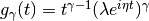
- class brian.hears.LinearGammachirp(source, f, time_constant, c, phase=0)
Bank of gammachirp filters with linear frequency sweeps and gamma envelope as described in Wagner et al. 2009, “Auditory responses in the barn owl’s nucleus laminaris to clicks: impulse response and signal analysis of neurophonic potential”, J. Neurophysiol.
The impulse response
is defined as follow
 where
where  corresponds to time_constant and
  to
phase (see definition of parameters).
to
phase (see definition of parameters).Those filters are implemented as FIR filters using truncated time representations of gammachirp functions as the impulse response. The impulse responses, which need to have the same length for every channel, have a duration of 15 times the biggest time constant. The length of the impulse response is therefore 15*max(time_constant)*sampling_rate. The impulse responses are normalized with respect to the transmitted power, i.e. the rms of the filter taps is 1.
Initialisation parameters:
- source
- Source sound or filterbank.
- f
- List or array of the sweep starting frequencies
(
 ).
). - time_constant
- Determines the duration of the envelope and consequently the length of the impulse response.
- c=1
- The glide slope (or sweep rate) given in Hz/second. The time-dependent instantaneous frequency is f+c*t and is therefore going upward when c>0 and downward when c<0. c can either be a scalar and will be the same for every channel or an array with the same length as f.
- phase=0
- Phase shift of the carrier.
Has attributes:
- length_impulse_response
- Number of samples in the impulse responses.
- impulse_response
- Array of shape (nchannels, length_impulse_response) with each row being an impulse response for the corresponding channel.
- class brian.hears.LinearGaborchirp(source, f, time_constant, c, phase=0)
Bank of gammachirp filters with linear frequency sweeps and gaussian envelope as described in Wagner et al. 2009, “Auditory responses in the barn owl’s nucleus laminaris to clicks: impulse response and signal analysis of neurophonic potential”, J. Neurophysiol.
The impulse response
is defined as follows:
 ,
where corresponds to time_constant and to
phase (see definition of parameters).
,
where corresponds to time_constant and to
phase (see definition of parameters).These filters are implemented as FIR filters using truncated time representations of gammachirp functions as the impulse response. The impulse responses, which need to have the same length for every channel, have a duration of 12 times the biggest time constant. The length of the impulse response is therefore 12*max(time_constant)*sampling_rate. The envelope is a gaussian function (Gabor filter). The impulse responses are normalized with respect to the transmitted power, i.e. the rms of the filter taps is 1.
Initialisation parameters:
- source
- Source sound or filterbank.
- f
- List or array of the sweep starting frequencies
(
 ).
). - time_constant
- Determines the duration of the envelope and consequently the length of the impluse response.
- c=1
- The glide slope (or sweep rate) given ins Hz/second. The time-dependent instantaneous frequency is f+c*t and is therefore going upward when c>0 and downward when c<0. c can either be a scalar and will be the same for every channel or an array with the same length as f.
- phase=0
- Phase shift of the carrier.
Has attributes:
- length_impulse_response
- Number of sample in the impulse responses.
- impulse_response
- Array of shape (nchannels, length_impulse_response) with each row being an impulse response for the corresponding channel.
- class brian.hears.IIRFilterbank(source, nchannels, passband, stopband, gpass, gstop, btype, ftype)
Filterbank of IIR filters. The filters can be low, high, bandstop or bandpass and be of type Elliptic, Butterworth, Chebyshev etc. The passband and stopband can be scalars (for low or high pass) or pairs of parameters (for stopband and passband) yielding similar filters for every channel. They can also be arrays of shape (1, nchannels) for low and high pass or (2, nchannels) for stopband and passband yielding different filters along channels. This class uses the scipy iirdesign function to generate filter coefficients for every channel.
See the documentation for scipy.signal.iirdesign for more details.
Initialisation parameters:
- samplerate
- The sample rate in Hz.
- nchannels
- The number of channels in the bank
- passband, stopband
- The edges of the pass and stop bands in Hz. For lowpass and highpass filters, in the case of similar filters for each channel, they are scalars and passband<stopband for low pass or stopband>passband for a highpass. For a bandpass or bandstop filter, in the case of similar filters for each channel, make passband and stopband a list with two elements, e.g. for a bandpass have passband=[200*Hz, 500*Hz] and stopband=[100*Hz, 600*Hz]. passband and stopband can also be arrays of shape (1, nchannels) for low and high pass or (2, nchannels) for stopband and passband yielding different filters along channels.
- gpass
- The maximum loss in the passband in dB. Can be a scalar or an array of length nchannels.
- gstop
- The minimum attenuation in the stopband in dB. Can be a scalar or an array of length nchannels.
- btype
- One of ‘low’, ‘high’, ‘bandpass’ or ‘bandstop’.
- ftype
- The type of IIR filter to design: ‘ellip’ (elliptic), ‘butter’ (Butterworth), ‘cheby1’ (Chebyshev I), ‘cheby2’ (Chebyshev II), ‘bessel’ (Bessel).
- class brian.hears.Butterworth(source, nchannels, order, fc, btype='low')
Filterbank of low, high, bandstop or bandpass Butterworth filters. The cut-off frequencies or the band frequencies can either be the same for each channel or different along channels.
Initialisation parameters:
- samplerate
- Sample rate.
- nchannels
- Number of filters in the bank.
- order
- Order of the filters.
- fc
- Cutoff parameter(s) in Hz. For the case of a lowpass or highpass filterbank, fc is either a scalar (thus the same value for all of the channels) or an array of length nchannels. For the case of a bandpass or bandstop, fc is either a pair of scalar defining the bandpass or bandstop (thus the same values for all of the channels) or an array of shape (2, nchannels) to define a pair for every channel.
- btype
- One of ‘low’, ‘high’, ‘bandpass’ or ‘bandstop’.
- class brian.hears.Cascade(source, filterbank, n)
Cascade of n times a linear filterbank.
Initialised with arguments:
- source
- Source of the new filterbank.
- filterbank
- Filterbank object to be put in cascade
- n
- Number of cascades
- class brian.hears.LowPass(source, fc)
Bank of 1st-order lowpass filters
The code is based on the code found in the Meddis toolbox. It was implemented here to be used in the DRNL cochlear model implementation.
Initialised with arguments:
- source
- Source of the filterbank.
- fc
- Value, list or array (with length = number of channels) of cutoff frequencies.
- class brian.hears.AsymmetricCompensation(source, f, b=1.019, c=1, ncascades=4)
Bank of asymmetric compensation filters.
Those filters are meant to be used in cascade with gammatone filters to approximate gammachirp filters (Unoki et al., 2001, Improvement of an IIR asymmetric compensation gammachirp filter, Acoust. Sci. & Tech.). They are implemented a a cascade of low order filters. The code is based on the implementation found in the AIM-MAT toolbox.
Initialised with arguments:
- source
- Source of the filterbank.
- f
- List or array of the cut off frequencies.
- b=1.019
- Determines the duration of the impulse response. Can either be a scalar and will be the same for every channel or an array with the same length as cf.
- c=1
- The glide slope when this filter is used to implement a gammachirp. Can either be a scalar and will be the same for every channel or an array with the same length as cf.
- ncascades=4
- The number of time the basic filter is put in cascade.
Auditory model library
- class brian.hears.DRNL(source, cf, type='human', param={})
Implementation of the dual resonance nonlinear (DRNL) filter as described in Lopez-Paveda, E. and Meddis, R., “A human nonlinear cochlear filterbank”, JASA 2001.
The entire pathway consists of the sum of a linear and a nonlinear pathway.
The linear path consists of a bank of bandpass filters (second order gammatone), a low pass function, and a gain/attenuation factor, g, in a cascade.
The nonlinear path is a cascade consisting of a bank of gammatone filters, a compression function, a second bank of gammatone filters, and a low pass function, in that order.
Initialised with arguments:
- source
- Source of the cochlear model.
- cf
- List or array of center frequencies.
- type
defines the parameters set corresponding to a certain fit. It can be either:
- type='human'
- The parameters come from Lopez-Paveda, E. and Meddis, R.., “A human nonlinear cochlear filterbank”, JASA 2001.
- type ='guinea pig'
- The parameters come from Summer et al., “A nonlinear filter-bank model of the guinea-pig cochlear nerve: Rate responses”, JASA 2003.
- param
- Dictionary used to overwrite the default parameters given in the original papers.
The possible parameters to change and their default values for humans (see Lopez-Paveda, E. and Meddis, R.,”A human nonlinear cochlear filterbank”, JASA 2001. for notation) are:
param['stape_scale']=0.00014
param['order_linear']=3
param['order_nonlinear']=3
from there on the parameters are given in the form
 where
cf is the center frequency:
where
cf is the center frequency:param['cf_lin_p0']=-0.067 param['cf_lin_m']=1.016 param['bw_lin_p0']=0.037 param['bw_lin_m']=0.785 param['cf_nl_p0']=-0.052 param['cf_nl_m']=1.016 param['bw_nl_p0']=-0.031 param['bw_nl_m']=0.774 param['a_p0']=1.402 param['a_m']=0.819 param['b_p0']=1.619 param['b_m']=-0.818 param['c_p0']=-0.602 param['c_m']=0 param['g_p0']=4.2 param['g_m']=0.48 param['lp_lin_cutoff_p0']=-0.067 param['lp_lin_cutoff_m']=1.016 param['lp_nl_cutoff_p0']=-0.052 param['lp_nl_cutoff_m']=1.016
- class brian.hears.DCGC(source, cf, update_interval=1, param={})
The compressive gammachirp auditory filter as described in Irino, T. and Patterson R., “A compressive gammachirp auditory filter for both physiological and psychophysical data”, JASA 2001.
Technical implementation details and notation can be found in Irino, T. and Patterson R., “A Dynamic Compressive Gammachirp Auditory Filterbank”, IEEE Trans Audio Speech Lang Processing.
The model consists of a control pathway and a signal pathway in parallel.
The control pathway consists of a bank of bandpass filters followed by a bank of highpass filters (this chain yields a bank of gammachirp filters).
The signal pathway consist of a bank of fix bandpass filters followed by a bank of highpass filters with variable cutoff frequencies (this chain yields a bank of gammachirp filters with a level-dependent bandwidth). The highpass filters of the signal pathway are controlled by the output levels of the two stages of the control pathway.
Initialised with arguments:
- source
- Source of the cochlear model.
- cf
- List or array of center frequencies.
- update_interval
- Interval in samples controlling how often the band pass filter of the signal pathway is updated. Smaller values are more accurate, but give longer computation times.
- param
- Dictionary used to overwrite the default parameters given in the original paper.
The possible parameters to change and their default values (see Irino, T. and Patterson R., “A Dynamic Compressive Gammachirp Auditory Filterbank”, IEEE Trans Audio Speech Lang Processing) are:
param['b1'] = 1.81
param['c1'] = -2.96
param['b2'] = 2.17
param['c2'] = 2.2
param['decay_tcst'] = .5*ms
param['lev_weight'] = .5
param['level_ref'] = 50.
param['level_pwr1'] = 1.5
param['level_pwr2'] = .5
param['RMStoSPL'] = 30.
param['frat0'] = .2330
param['frat1'] = .005
param['lct_ERB'] = 1.5  #value of the shift in ERB frequencies
param['frat_control'] = 1.08
param['order_gc']=4
param['ERBrate']= 21.4*log10(4.37*cf/1000+1) # cf is the center frequency
param['ERBwidth']= 24.7*(4.37*cf/1000 + 1)
- class brian.hears.MiddleEar(source, gain=1, **kwds)
Implements the middle ear model from Tan & Carney (2003) (linear filter with two pole pairs and one double zero). The gain is normalized for the response of the analog filter at 1000Hz as in the model of Tan & Carney (their actual C code does however result in a slightly different normalization, the difference in overall level is about 0.33dB (to get exactly the same output as in their model, set the gain parameter to 0.962512703689).
Tan, Q., and L. H. Carney. “A Phenomenological Model for the Responses of Auditory-nerve Fibers. II. Nonlinear Tuning with a Frequency Glide”. The Journal of the Acoustical Society of America 114 (2003): 2007.
- class brian.hears.TanCarney(source, cf, update_interval=1, param=None)
Class implementing the nonlinear auditory filterbank model as described in Tan, G. and Carney, L., “A phenomenological model for the responses of auditory-nerve fibers. II. Nonlinear tuning with a frequency glide”, JASA 2003.
The model consists of a control path and a signal path. The control path controls both its own bandwidth via a feedback loop and also the bandwidth of the signal path.
Initialised with arguments:
- source
- Source of the cochlear model.
- cf
- List or array of center frequencies.
- update_interval
- Interval in samples controlling how often the band pass filter of the signal pathway is updated. Smaller values are more accurate but increase the computation time.
- param
- Dictionary used to overwrite the default parameters given in the original paper.
- class brian.hears.ZhangSynapse(source, CF, n_per_channel=1, params=None)
A FilterbankGroup that represents an IHC-AN synapse according to the Zhang et al. (2001) model. The source should be a filterbank, producing V_ihc (e.g. TanCarney). CF specifies the characteristic frequencies of the AN fibers. params overwrites any parameters values given in the publication.
The group emits spikes according to a time-varying Poisson process with absolute and relative refractoriness (probability of spiking is given by state variable R). The continuous probability of spiking without refractoriness is available in the state variable s.
The n_per_channel argument can be used to generate multiple spike trains for every channel.
If all you need is the state variable s, you can use the class ZhangSynapseRate instead which does not simulate the spike-generating Poisson process.
For details see: Zhang, X., M. G. Heinz, I. C. Bruce, and L. H. Carney. “A Phenomenological Model for the Responses of Auditory-nerve Fibers: I. Nonlinear Tuning with Compression and Suppression”. The Journal of the Acoustical Society of America 109 (2001): 648.
Filterbank group
- class brian.hears.FilterbankGroup(filterbank, targetvar, *args, **kwds)
Allows a Filterbank object to be used as a NeuronGroup
Initialised as a standard NeuronGroup object, but with two additional arguments at the beginning, and no N (number of neurons) argument. The number of neurons in the group will be the number of channels in the filterbank. (TODO: add reference to interleave/serial channel stuff here.)
- filterbank
- The Filterbank object to be used by the group. In fact, any Bufferable object can be used.
- targetvar
- The target variable to put the filterbank output into.
One additional keyword is available beyond that of NeuronGroup:
- buffersize=32
- The size of the buffered segments to fetch each time. The efficiency depends on this in an unpredictable way, larger values mean more time spent in optimised code, but are worse for the cache. In many cases, the default value is a good tradeoff. Values can be given as a number of samples, or a length of time in seconds.
Note that if you specify your own Clock, it should have 1/dt=samplerate.
Functions
- brian.hears.erbspace(*args, **kwds)
Returns the centre frequencies on an ERB scale.
- low, high
- Lower and upper frequencies
- N
- Number of channels
- earQ=9.26449, minBW=24.7, order=1
- Default Glasberg and Moore parameters.
- brian.hears.asymmetric_compensation_coeffs(samplerate, fr, filt_b, filt_a, b, c, p0, p1, p2, p3, p4)
This function is used to generated the coefficient of the asymmetric compensation filter used for the gammachirp implementation.
Plotting
- brian.hears.log_frequency_xaxis_labels(ax=None, freqs=None)
Sets tick positions for log-scale frequency x-axis at sensible locations.
Also uses scalar representation rather than exponential (i.e. 100 rather than 10^2).
- ax=None
- The axis to set, or uses gca() if None.
- freqs=None
- Override the default frequency locations with your preferred tick locations.
See also: log_frequency_yaxis_labels().
Note: with log scaled axes, it can be useful to call axis('tight') before setting the ticks.
- brian.hears.log_frequency_yaxis_labels(ax=None, freqs=None)
Sets tick positions for log-scale frequency x-axis at sensible locations.
Also uses scalar representation rather than exponential (i.e. 100 rather than 10^2).
- ax=None
- The axis to set, or uses gca() if None.
- freqs=None
- Override the default frequency locations with your preferred tick locations.
See also: log_frequency_yaxis_labels().
Note: with log scaled axes, it can be useful to call axis('tight') before setting the ticks.
HRTFs
- class brian.hears.HRTF(hrir_l, hrir_r=None)
Head related transfer function.
Attributes
- impulse_response
- The pair of impulse responses (as stereo Sound objects)
- fir
- The impulse responses in a format suitable for using with FIRFilterbank (the transpose of impulse_response).
- left, right
- The two HRTFs (mono Sound objects)
- samplerate
- The sample rate of the HRTFs.
Methods
- apply(sound)
Returns a stereo Sound object formed by applying the pair of HRTFs to the mono sound input. Equivalently, you can write hrtf(sound) for hrtf an HRTF object.
- filterbank(source, **kwds)
Returns an FIRFilterbank object that can be used to apply the HRTF as part of a chain of filterbanks.
You can get the number of samples in the impulse response with len(hrtf).
- class brian.hears.HRTFSet(data, samplerate, coordinates)
A collection of HRTFs, typically for a single individual.
Normally this object is created automatically by an HRTFDatabase.
Attributes
- hrtf
- A list of HRTF objects for each index.
- num_indices
- The number of HRTF locations. You can also use len(hrtfset).
- num_samples
- The sample length of each HRTF.
- fir_serial, fir_interleaved
- The impulse responses in a format suitable for using with FIRFilterbank, in serial (LLLLL...RRRRR....) or interleaved (LRLRLR...).
Methods
- subset(condition)
Generates the subset of the set of HRTFs whose coordinates satisfy the condition. This should be one of: a boolean array of length the number of HRTFs in the set, with values of True/False to indicate if the corresponding HRTF should be included or not; an integer array with the indices of the HRTFs to keep; or a function whose argument names are names of the parameters of the coordinate system, e.g. condition=lambda azim:azim<pi/2.
- filterbank(source, interleaved=False, **kwds)
Returns an FIRFilterbank object which applies all of the HRTFs in the set. If interleaved=False then the channels are arranged in the order LLLL...RRRR..., otherwise they are arranged in the order LRLRLR....
You can access an HRTF by index via hrtfset[index], or by its coordinates via hrtfset(coord1=val1, coord2=val2).
Initialisation
- data
- An array of shape (2, num_indices, num_samples) where data[0,:,:] is the left ear and data[1,:,:] is the right ear, num_indices is the number of HRTFs for each ear, and num_samples is the length of the HRTF.
- samplerate
- The sample rate for the HRTFs (should have units of Hz).
- coordinates
- A record array of length num_indices giving the coordinates of each HRTF. You can use make_coordinates() to help with this.
- class brian.hears.HRTFDatabase(samplerate=None)
Base class for databases of HRTFs
Should have an attribute ‘subjects’ giving a list of available subjects, and a method load_subject(subject) which returns an HRTFSet for that subject.
The initialiser should take (optional) keywords:
- samplerate
- The intended samplerate (resampling will be used if it is wrong). If left unset, the natural samplerate of the data set will be used.
- brian.hears.make_coordinates(**kwds)
Creates a numpy record array from the keywords passed to the function. Each keyword/value pair should be the name of the coordinate the array of values of that coordinate for each location. Returns a numpy record array. For example:
coords = make_coordinates(azimuth=[0, 30, 60, 0, 30, 60],
                          elevation=[0, 0, 0, 30, 30, 30])
print coords['azimuth']
- class brian.hears.IRCAM_LISTEN(basedir, compensated=False, samplerate=None)
HRTFDatabase for the IRCAM LISTEN public HRTF database.
For details on the database, see the website.
The database object can be initialised with the following arguments:
- basedir
- The directory where the database has been downloaded and extracted, e.g. r'D:\HRTF\IRCAM'. Multiple directories in a list can be provided as well (e.g IRCAM and IRCAM New).
- compensated=False
- Whether to use the raw or compensated impulse responses.
- samplerate=None
- If specified, you can resample the impulse responses to a different samplerate, otherwise uses the default 44.1 kHz.
The coordinates are pairs (azim, elev) where azim ranges from 0 to 345 degrees in steps of 15 degrees, and elev ranges from -45 to 90 in steps of 15 degrees. After loading the database, the attribute ‘subjects’ gives all the subjects number that were detected as installed.
Obtaining the database
The database can be downloaded here. Each subject archive should be extracted to a folder (e.g. IRCAM) with the names of the subject, e.g. IRCAM/IRC_1002, etc.
- class brian.hears.HeadlessDatabase(n=None, azim_max=1.5707963267948966, diameter=0.22308 * metre, itd=None, samplerate=None, fractional_itds=False)
Database for creating HRTFSet with artificial interaural time-differences
Initialisation keywords:
- n, azim_max, diameter
- Specify the ITDs for two ears separated by distance diameter with no head. ITDs corresponding to n angles equally spaced between -azim_max and azim_max are used. The default diameter is that which gives the maximum ITD as 650 microseconds. The ITDs are computed with the formula diameter*sin(azim)/speed_of_sound_in_air. In this case, the generated HRTFSet will have coordinates of azim and itd.
- itd
- Instead of specifying the keywords above, just give the ITDs directly. In this case, the generated HRTFSet will have coordinates of itd only.
- fractional_itds=False
- Set this to True to allow ITDs with a fractional multiple of the timestep 1/samplerate. Note that the filters used to do this are not perfect and so this will introduce a small amount of numerical error, and so shouldn’t be used unless this level of timing precision is required. See FractionalDelay for more details.
To get the HRTFSet, the simplest thing to do is just:
hrtfset = HeadlessDatabase(13).load_subject()
The generated ITDs can be returned using the itd attribute of the HeadlessDatabase object.
If fractional_itds=False then Note that the delays induced in the left and right channels are not symmetric as making them so wastes half the samplerate (if the delay to the left channel is itd/2 and the delay to the right channel is -itd/2). Instead, for each channel either the left channel delay is 0 and the right channel delay is -itd (if itd<0) or the left channel delay is itd and the right channel delay is 0 (if itd>0).
If fractional_itds=True then delays in the left and right channels will be symmetric around a global offset of delay_offset.
Base classes
Useful for understanding more about the internals.
- class brian.hears.Bufferable
Base class for Brian.hears classes
Defines a buffering interface of two methods:
- buffer_init()
- Initialise the buffer, should set the time pointer to zero and do any other initialisation that the object needs.
- buffer_fetch(start, end)
- Fetch the next samples start:end from the buffer. Value returned should be an array of shape (end-start, nchannels). Can throw an IndexError exception if it is outside the possible range.
In addition, bufferable objects should define attributes:
- nchannels
- The number of channels in the buffer.
- samplerate
- The sample rate in Hz.
By default, the class will define a default buffering mechanism which can easily be extended. To extend the default buffering mechanism, simply implement the method:
- buffer_fetch_next(samples)
- Returns the next samples from the buffer.
The default methods for buffer_init() and buffer_fetch() will define a buffer cache which will get larger if it needs to to accommodate a buffer_fetch(start, end) where end-start is larger than the current cache. If the filterbank has a minimum_buffer_size attribute, the internal cache will always have at least this size, and the buffer_fetch_next(samples) method will always get called with samples>=minimum_buffer_size. This can be useful to ensure that the buffering is done efficiently internally, even if the user request buffered chunks that are too small. If the filterbank has a maximum_buffer_size attribute then buffer_fetch_next(samples) will always be called with samples<=maximum_buffer_size - this can be useful for either memory consumption reasons or for implementing time varying filters that need to update on a shorter time window than the overall buffer size.
The following attributes will automatically be maintained:
- self.cached_buffer_start, self.cached_buffer_end
- The start and end of the cached segment of the buffer
- self.cached_buffer_output
- An array of shape ((cached_buffer_end-cached_buffer_start, nchannels) with the current cached segment of the buffer. Note that this array can change size.
- class brian.hears.Filterbank(source)
Generalised filterbank object
Documentation common to all filterbanks
Filterbanks all share a few basic attributes:
- source
The source of the filterbank, a Bufferable object, e.g. another Filterbank or a Sound. It can also be a tuple of sources. Can be changed after the object is created, although note that for some filterbanks this may cause problems if they do make assumptions about the input based on the first source object they were passed. If this is causing problems, you can insert a dummy filterbank (DoNothingFilterbank) which is guaranteed to work if you change the source.
- nchannels
The number of channels.
- samplerate
The sample rate.
- duration
The duration of the filterbank. If it is not specified by the user, it is computed by finding the maximum of its source durations. If these are not specified a KeyError will be raised (for example, using OnlineSound as a source).
To process the output of a filterbank, the following method can be used:
- process(func=None, duration=None, buffersize=32)
Returns the output of the filterbank for the given duration.
- func
- If a function is specified, it should be a function of one or two arguments that will be called on each filtered buffered segment (of shape (buffersize, nchannels) in order. If the function has one argument, the argument should be buffered segment. If it has two arguments, the second argument is the value returned by the previous application of the function (or 0 for the first application). In this case, the method will return the final value returned by the function. See example below.
- duration=None
- The length of time (in seconds) or number of samples to process. If no func is specified, the method will return an array of shape (duration, nchannels) with the filtered outputs. Note that in many cases, this will be too large to fit in memory, in which you will want to process the filtered outputs online, by providing a function func (see example below). If no duration is specified, the maximum duration of the inputs to the filterbank will be used, or an error raised if they do not have durations (e.g. in the case of OnlineSound).
- buffersize=32
- The size of the buffered segments to fetch, as a length of time or number of samples. 32 samples typically gives reasonably good performance.
For example, to compute the RMS of each channel in a filterbank, you would do:
def sum_of_squares(input, running_sum_of_squares):
    return running_sum_of_squares+sum(input**2, axis=0)
rms = sqrt(fb.process(sum_of_squares)/nsamples)
Alternatively, the buffer interface can be used, which is described in more detail below.
Filterbank also defines arithmetical operations for +, -, *, / where the other operand can be a filterbank or scalar.
Details on the class
This class is a base class not designed to be instantiated. A Filterbank object should define the interface of Bufferable, as well as defining a source attribute. This is normally a Bufferable object, but could be an iterable of sources (for example, for filterbanks that mix or add multiple inputs).
The buffer_fetch_next(samples) method has a default implementation that fetches the next input, and calls the buffer_apply(input) method on it, which can be overridden by a derived class. This is typically the easiest way to implement a new filterbank. Filterbanks with multiple sources will need to override this default implementation.
There is a default __init__ method that can be called by a derived class that sets the source, nchannels and samplerate from that of the source object. For multiple sources, the default implementation will check that each source has the same number of channels and samplerate and will raise an error if not.
There is a default buffer_init() method that calls buffer_init() on the source (or list of sources).
Example of deriving a class
The following class takes N input channels and sums them to a single output channel:
class AccumulateFilterbank(Filterbank):
    def __init__(self, source):
        Filterbank.__init__(self, source)
        self.nchannels = 1
    def buffer_apply(self, input):
        return reshape(sum(input, axis=1), (input.shape[0], 1))
Note that the default Filterbank.__init__ will set the number of channels equal to the number of source channels, but we want to change it to have a single output channel. We use the buffer_apply method which automatically handles the efficient cacheing of the buffer for us. The method receives the array input which has shape (bufsize, nchannels) and sums over the channels (axis=1). It’s important to reshape the output so that it has shape (bufsize, outputnchannels) so that it can be used as the input to subsequent filterbanks.
- class brian.hears.BaseSound
Base class for Sound and OnlineSound
- class brian.hears.OnlineSound
Options
There are several relevant global options for Brian hears. In particular, activating scipy Weave support with the useweave=True will give considerably faster linear filtering. See Preferences and Compiled code for more details.
Class diagram
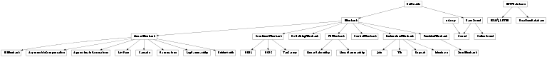
![]()
Project Versions
RTD Search
Full-text doc search.